LoRA Training Dynamics

Trying to get LoRA to match FullFT

A few months ago, I was reading LoRA without Regret, and the result that the optimal learning rate for LoRA is 10x the optimal learning rate for FullFT (Figure 2) stuck out to me as very mysterious. Particularly, this result is independent of the model hidden dimension $d$. Imagine you have two weight matrices, one is $2048\times 2048$, and the other is $8192\times 8192$, and you train a rank-1 LoRA adapter on top of them. Even though the ratio between the FullFT rank and the LoRA rank is drastically different, the ratio between the optimal learning rates is the same. Taking this argument to its limit, as $d \rightarrow \infty$, you would think that fixed-size the LoRA adapter does progressively worse and needs a progressively larger learning rate, but it doesn’t. How does this make any sense?

Background on LoRA

In LoRA, we replace the weight matrix $W$ with $W’ = W + \gamma AB$, where $W$ is the fixed weight matrix from a pretrained model, $A$ and $B$ are trainable low-rank matrices, and $\gamma$ is a scaling factor. LoRA attempts to capture a low-dimensional representation of the weight update imparted during finetuning.

To keep the optimal learning rate invariant to LoRA rank during training, $\gamma$ is typically parametrized so that $\gamma \propto \frac{1}{r}$ when using Adam as your optimizer, where $r$ is the rank of the LoRA adapter.

The proof that this works is fairly simple. We write the LoRA update matrix as $W_{\text{LoRA}} = (1/r)BA = (1/r)\sum_{i=1}^r b_i a_i^\top$, where each pair $(b_i, a_i)$ is independently initialized. During the first optimization step, the vectors $b_i$ and $a_i$ each receive small parameter updates, which we denote by $U_{b_i} = b_i^{(1)} - b_i^{(0)}$ and $U_{a_i} = a_i^{(1)} - a_i^{(0)}$. The resulting change to the outer product $b_i a_i^\top$ is the matrix

\[U_{(b_i a_i^\top)} = b_i^{(1)} a_i^{(1)\top} - b_i^{(0)} a_i^{(0)\top} \propto \nabla_{b_i} L \; a_i^{(0)\top} + b_i^{(0)} \nabla_{a_i} L^\top\]

The update to the entire LoRA matrix is the sum of these contributions, $U_{W_{\text{LoRA}}} = (1/r)\sum_{i=1}^r U_{(b_i a_i^\top)}$. Because all $(b_i^{(0)}, a_i^{(0)})$ pairs are drawn i.i.d. from the same initialization distribution, the gradients $\nabla_{b_i} L$ and $\nabla_{a_i} L$ at step 1 have identical distributions across ranks, and therefore each rank-1 update $U_{(b_i a_i^\top)}$ has the same expectation. If we denote this common expectation by $\mu$, then $\mathbb{E}\left[U_{W_{\text{LoRA}}}\right] = (1/r)\sum_{i=1}^r \mathbb{E}\left[U_{(b_i a_i^\top)}\right] = \mu$. Since the expected update contributed by each rank-1 component is independent of the rank, the total LoRA update is simply the average of $r$ identically distributed terms.

When you are using SGD, the analysis is a bit different. In this case, the expected update scales with the gradient, and the gradient is proportional to $\gamma$. In Adam, the update is in the direction of the normalized gradient, so the direction of the gradient is what matters, not its magnitude (a useful intuition to have is that Adam is approximately SignGD). Thus, under SGD, the expected update in a rank-$r$ adapter, $E\left[U^r_{(b_i a_i^\top)}\right]$, is equal to $\frac{\gamma(r)}{\gamma(1)} \mathbb{E}\left[U^1_{(b_i a_i^\top)}\right]$.

\[\mathbb{E}\left[U_{W_{\text{LoRA}}}\right] = \gamma(r) \mathbb{E}\left[ \sum_{i=1}^r U^r_{b_i a_i^\top} \right] \\ = \frac{\gamma(r)^2}{\gamma(1)} \mathbb{E}\left[ \sum_{i=1}^r U^1_{b_i a_i^\top} \right] \\ = \gamma(1) \mathbb{E}\left[U^1_{b_i a_i^\top}\right]\]

To keep the expected update constant, we need $\gamma(r) \propto \frac{1}{\sqrt{r}}$.

Thus, in practice, we parametrize $W’ = W + \frac{\alpha}{r} BA$ for Adam and $W’ = W + \frac{\alpha}{\sqrt{r}} BA$ for SGD, where $\alpha$ is a hyperparameter. Additionally, we usually initialize $B$ to zero and randomly initialize $A$. Now, we have a parametrization of LoRA such that the optimal learning rate is rank-invariant, which enables us to reason about the relationship between FullFT and LoRA learning rates.

An Incorrect Starting Point

The Blogpost

The blogpost attempts to derive a relationship between the FullFT and LoRA learning rates. They start with the assumption that full-rank LoRA is directly comparable to FullFT. To be honest, I didn’t fully understand their derivation, but this is my best approximation of it:

They assume that full finetuning can be approximated as $W=W_0+BA$ with $B\in\mathbb{R}^{d\times (d/2)}$, $A\in\mathbb{R}^{(d/2)\times d}$, using learning rate $\mathrm{LR}_{\mathrm{FullFT}}$. This choice of dimensions is to match the number of parameters between FullFT and a hypothetical full-rank LoRA.

To match the effective learning rates, they set

\[\text{LR}_{\text{FullFT}} = \frac{\alpha}{d / 2} \text{LR}_{\text{LoRA}}\]

which gives:

\[\frac{\text{LR}_{\text{LoRA}}}{\text{LR}_{\text{FullFT}}}=\frac{d}{2\alpha}.\]

However, this gives a dependence on $d$! This contradicts the empirical observation that the learning rate ratio is independent of the hidden dimension.

Another analysis

I will present yet another way of arriving at a similar result when using SGD, that is still rather wrong but also interesting.

Typically during training, $B$ is initialized to zero, while $A$ is initialized through some form of Kaiming initialization. Thus, early on, most of the update comes from $B$ (the gradients flowing to $A$ are close to zero). This means $U_{b_i a_i^\top} \approx U_{b_i} a_i^\top$.

Suppose $G$ is the gradient flowing to the total LoRA matrix $BA$. Then, $U_{b_i} \propto G_{b_i} = G a_i$. The total amount by which the update moves in the direction of the gradient is $\langle U_{b_i} a_i a_i^\top, G \rangle \propto \langle G a_i a_i^\top, G\rangle = \lVert G a_i\rVert_2^2$.

If we consider a single row of $G$, which I denote as $g^j$, then the amount by which the update moves in the direction of the gradient for that row is $\lVert g^j \rVert^2 \lVert a_i \rVert^2 \cos^2{\theta}$, where $\theta$ is the angle between $a_i$ and $g^j$. So, if your LoRA matrix is more aligned with the gradient, your adapters will receive larger updates.

Assuming $a_i$ is a randomly initialized $d$-dimensional normal vector, $\mathbb{E}[\cos^2{\theta}] \propto \frac{1}{d}$. Thus, to get the same total movement in the direction of the gradient under LoRA, you would need a $d$ times larger learning rate!

This analysis also incorrectly predicts a dependence on $d$, which contradicts the empirical evidence.

LoRA Aligns with the Gradient

It is clear empirically that both of the analyses above are false. So what is going on?

The key insight is that the incorrect assumption we have been making is that $a_i$ remains unaligned with the gradient. For simplicity, let’s assume that we are looking at a rank-1 LoRA, trained under SGD. While it is true that $a_i$ starts unaligned at the very beginning of training, within a few steps, $a_i$ will actually align to become very close to the top right singular vector of $G$!

To get a sense of why this happens, first consider that since $b_i$ is initialized to zero, it will always be in the direction of the projected gradient: $b_i \propto -G a_i$.

Thus, the update to $a_i$ is: \(a_i = a_i - \eta G^\top b_i = a_i + \eta G^\top G a_i\)

Plugging in the SVD decomposition $G = U \Sigma V^\top$, we get: \(a_i = a_i + \eta G^\top G a_i = (I + \eta V \Sigma^2 V^\top) a_i\)

This update is reminiscent of power iteration. The overall effect is that the top singular vectors will become more dominant over time, since the update is scaling each singular vector by a factor of $1 + \eta \lambda_i^2$, where $\lambda_i$ are the singular values. The larger singular values get amplified more, causing $a_i$ to align with the top right singular vector.

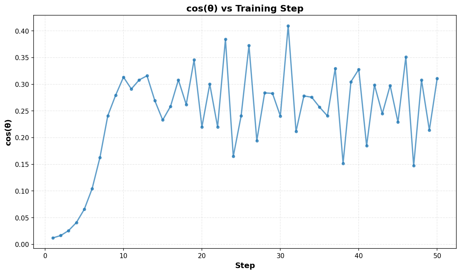
Empirically, you can plot the angle $\theta$ between $a_i$ and the top singular vector of $G$ over time. We can see that $\cos(\theta)$ starts quite small (meaning $a_i$ is initially unaligned), and shoots up within a few steps (meaning $a_i$ quickly aligns with the top singular vector)!

It can never quite perfectly align with $G$ because $G$ is noisy and evolves during training, and the LoRA parameters are constantly chasing its new low-rank approximation. (For reference, I’m training Llama-3.2-1B on the Tulu-3 dataset)

This analysis gives some insight into how $BA$ is able to evolve into a low-rank approximation of $G$. While LoRA is typically seen as a low-rank approximation of the FullFT weight update, it can also be thought of as a low-rank approximation of the gradient; I haven’t seen this perspective used much and I think it is quite insightful.

The gradient is typically very low-rank once you get to the stage of finetuning, which explains why LoRA is able to perform so well. It also explains when it performs badly: when $BA$ has finished aligning with a previous gradient direction and is no longer aligned with the current subspace of $G$, that is roughly when you should absorb $BA$ into $W$ and then reinitialize $BA$ through a technique like ReLoRA. The full update matrix $\Delta W$ can be of arbitrarily high rank: as long as the gradients at any point in training are still low-rank, ReLoRA efficiently captures all of the information it has.

Coming back to the analysis in the previous section, let’s suppose $G$ is a rank-1 matrix $u \lambda v^\top$. Then, $\lVert G a_i \rVert_2^2$, assuming $a_i \approx v$, is $\lVert u \lambda \rVert_2^2 = \lambda^2$. Thus, the magnitude of the update in the direction of the gradient under rank-1 LoRA matches that of FullFT.

Now of course there are some simplifying assumptions here (as shown above, $a_i$ doesn’t quite become $v$, and we are looking at SGD instead of Adam), so this analysis doesn’t quite explain the factor of $10$. However, it hopefully convinces you that a relationship between FullFT and LoRA learning rates that involves $d$ doesn’t actually make sense.

After I independently discovered this, I realized there is a wonderful paper that explains all of this with more rigor. A clear sign that I still need to be reading more papers!

An Improved Initialization

This analysis also sparks a cool idea: instead of forcing $A$ to evolve into the top right singular vector of $G$, what if you just initialize it so? You can calculate the SVD from the first step of finetuning, and then reinitialize $A$ to the top right singular vector.

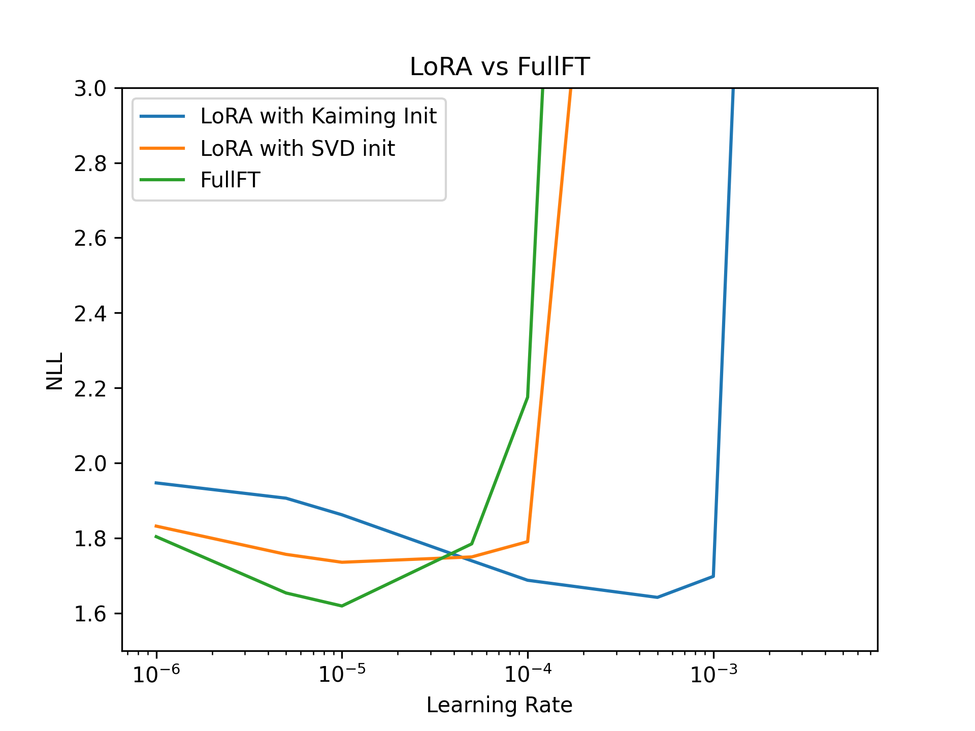
I compared this approach to standard Kaiming initialization and FullFT, using Adam as my optimizer and $\alpha=32$ to match the setting of Thinking Machine’s experiment. I’m training a rank-1 LoRA for Llama-3.2-3B on the Tulu-3 Dataset, and the full reproduction code can be found here. This is something of a reproduction of a result in some other papers that introduce the idea. This improved initialization results in optimal learning rates that match FullFT, suggesting that its early training dynamics are a better approximation of it!

Note that I only ran training for 100 steps: while I have not tried it, I suspect that for very long training runs, the results would not be as clean. This is because LoRA will fully learn the relevant subspaces of $G$ and so the gradients will evolve into new subspaces, at which point this initialization no longer helps. It only helps while $G$ remains in the subspace of the first finetuning step.

Acknowledgements

Thanks to Adam Zweiger and Atticus Wang for some ideas that prompted this post, and thanks to Nathan Wang for giving feedback on a draft. I’m also extremely grateful to Modal for sponsoring compute and making it possible to play around with a B200 all day!

---

If you found this useful, please cite this as:

Goel, Tarushii (Nov 2025). LoRA Training Dynamics. https://tarushii-g.github.io.

or as a BibTeX entry:

@article{goel2025lora-training-dynamics,
  title   = {LoRA Training Dynamics},
  author  = {Goel, Tarushii},
  year    = {2025},
  month   = {Nov},
  url     = {https://tarushii-g.github.io/blog/2025/lora-training/}
}